Rebrained!

Python Monte Carlo graphs

I wanted to plot the paths of my Monte Carlo simulation of Black Scholes in my previous post.

Using iPython started with the –pylab flag, it’s pretty easy.

from math import exp
from random import gauss
St0=41.75
rate=.0535
vol=.34
trials=100
for trials in range(trials):
    prices=[St0]
    for day in range(time):
        prices.append(prices[day]*exp((rate-.5*vol**2)*(1.0/365)+vol*(1.0/365)**.5*gauss(0,1)))
    plot(prices)

The code above gives me this nice graph of the stock price “walks” over time:

Things get a little crazier when I make the volatility 3.4 instead of .34:

Using my one line blackscholes function from the previous post, how does the price of the option change as we increase the volatility from .34 to 3.4?

How does the price of the option change as we increase the number of days to expiry?

Posted in finance, programming | No Comments »

Black Scholes Monte Carlo in Python

The Black Scholes formula is a partial differential equation that can be used to price the present value of an option under certain assumptions. As with everything, you can read all about it in Wikipedia.

It turns that that figuring out the present value of an option is also a good candidate for a Monte Carlo approach. I went through a very simple example of Monte Carlo in my previous post.

Let’s say I have a put option on a particular stock which will pay out at a certain time in the future (the expiry date for European style options, which this approach is restricted to). The payout will be how much less than a given strike price the stock is at the expiry date. If the stock is over that strike price at the expiry date, it’s worth zero.

In the Black Scholes model, stock prices are assumed to fluctuate, or evolve, according to the formula below:

By a process of discretization, we can chop the time interval above into smaller chunks (say 1 day). We can then assume that the brownian motion over this short period will be a normal (gaussian) distribution with a mean of 0 and a variance of the time interval. This is all nicely explained in Wikipedia here and yields the discretized formula:

So turning that into some python code, to find tomorrow’s stock price from today’s price and a given volatility and riskless rate:

>>> from math import exp
>>> from random import gauss
>>> St0=41.75
>>> rate=.0535
>>> vol=.34
>>> delta=exp((rate-.5*vol**2)*(1.0/365)+vol*(1.0/365)**.5*gauss(0,1))
>>> St0+delta
42.747744977337405
>>>

If we wanted to “walk” this price forward for multiple days (say there’s 61 days to expiry), we could add the following to the above:

>>> time=61
>>> delta=lambda x: \
... x*exp((rate-.5*vol**2)*(1.0/365)+vol*(1.0/365)**.5*gauss(0,1))-x
>>> ST=reduce(lambda x,y: x+delta(x),range(time),St0)
>>> ST
38.89640199216139

So what’s the value of this put option if the strike price is $45?

>>> strike=45
>>> ST=lambda: reduce(lambda x,y: x+delta(x),range(time),St0)
>>> max(0,strike-ST())
6.323401387138546
>>> max(0,strike-ST())
12.364539627699976
>>> max(0,strike-ST())
6.9642390525076365
>>> max(0,strike-ST())
0
>>> max(0,strike-ST())
8.417050607508223
>>> max(0,strike-ST())
0
>>>

You see that the price of the option varies wildly each time I run this. This is where the Monte Carlo method comes in. I want to run multiple trials of the option value, then average them to get a price that will converge on the Black Scholes price.

A little more python code, and you have it:

>>> trials=10000
>>> reduce(lambda x,y: x+max(0,strike-ST()),range(trials))/trials
4.147540635574047
>>>

So this put option is worth a little over $4 today.

Sorry about the overuse of reduce and lambda functions – I’m kinda smitten by them today for some reason.

Here’s the above nicely formatted:

from math import exp
from random import gauss
rate=.0535
vol=.34
delta=lambda x:x*exp((rate-.5*vol**2)*(1.0/365)+vol*(1.0/365)**.5*gauss(0,1))-x
St0=41.75
time=61
ST=lambda: reduce(lambda x,y: x+delta(x),range(time),St0)
strike=45
trials=10000
print reduce(lambda x,y: x+max(0,strike-ST()),range(trials))/trials

A friend of mine – Ben – gave me the idea of a function with a custom payout so you can call it with a call, put or other kind of payout (it defaults to a call payout). He’d also I think done a version of it in one line, so here’s my attempt:

from random import gauss
from math import exp
def blackscholes(St0,strike,riskless,vol,time,trials,payout=lambda strike,ST: max(ST-strike,0)):
        return reduce(lambda x,y: x+payout(strike,reduce(lambda x,y: x*exp((riskless-.5*vol**2)*(1.0/365) + vol*(1.0/365)**.5*gauss(0,1)),range(time),St0)),range(trials))/trials

To run this function with the same put example above:

>>> blackscholes(41.75,45,.0535,.34,61,10000,lambda strike,ST:max(strike-ST,0))
>>> 4.195682577752359

By the way, the example above was taken from the Basic Black Scholes book, chapter 5, by Timothy Crack, which I would recommend.

Posted in finance, mathematics, programming | 1 Comment »

Python Monte Carlo

Monte Carlo is a simulation method that can be useful in solving problems that are difficult to solve analytically.

Here’s an interesting application of the technique to estimate the value of pi.

Consider a circular dartboard placed against a square backing, with the sides of the square perfectly touching the circle tangentially at the top, bottom, left and right.

If you throw a dart blindly inside of the square, what are the chances the dart will actually land inside the circle?

Assuming the radius of the circle is r, it is:

= area of circle / area of square

= (pi * r ^ 2) / (4 * r ^ 2)

= pi / 4

So the chances of hitting the circle are pi / 4.   In other words:

pi = 4 * the chances of hitting the circle.

So let’s set up a Monte Carlo simulation to work out the probability of getting the dart inside of the circle.  

To do this, let’s think of the quarter circle below:

Note that the chances of hitting the quarter circle inside of its square is the same as hitting the larger circle inside of the bigger square.   How can we easily simulate hitting the quarter circle?  We can obtain two random numbers between  0 and 1, representing the x and y coordinates of a point with the origin at the circle’s center.  If the distance between this point and the origin is less than 1, then we’re inside the quarter circle.  Otherwise we’re outside it.  If we simulate this enough times, and multiply the percentage of times we’re inside the circle by 4, we should converge on the value of pi.

Here’s a short python script that simulates this:

>>> from random import random
>>> reduce(lambda x,y:x+y,map(lambda x:(random()**2+random()**2)**.5<1,range(100
0000)))/1000000.0*4
3.1411799999999999
>>>

EDIT 12/4/2011
Thanks curious reader, I guess you’re right, a filter is a little simpler:

>>> from random import random
>>> len(filter(lambda x:(random()**2+random()**2)**.5<1,range(1000000)))/1000000.0*4
3.14064
>>>

Not to be picky, but don’t forget the “.0″ at the end of the last 1000000 in your list comprehension solution.

Posted in programming | 3 Comments »

Prime numbers and Numpy – Python

I’ve been looking at the element-wise operations in Numpy arrays. The code below generates 100K primes in about 1.3 secs on my laptop.

import numpy
import math
def prime(upto=100):
    return filter(lambda num: (num % numpy.arange(2,1+int(math.sqrt(num)))).all(), range(2,upto+1))

>>> prime()
[2, 3, 5, 7, 11, 13, 17, 19, 23, 29, 31, 37, 41, 43, 47, 53, 59, 61, 67, 71, 73, 79, 83, 89, 97]
>>>

Similiar code that uses a for loop runs about 5 times longer for 100K primes, about 7 secs:

import numpy
import math
def prime2(upto=100):
    return filter(lambda num: numpy.array([num % factor for factor in range(2,1+int(math.sqrt(num)))]).all(), range(2,upto+1))

By not including even numbers, the original code can be optimized to run in half the time again, about .7 secs for 100K primes.

import numpy
import math
def prime3(upto=100):
    return [2]+filter(lambda num: (num % numpy.arange(3,1+int(math.sqrt(num)),2)).all(), range(3,upto+1,2))

The above code is not the fastest implementation, but illustrative of using the element-wise operations in Numpy arrays rather than looping through a list.

We can write faster code by breaking after finding the first modulo equal zero condition. The code below runs in about .4 seconds for 100K primes:

import numpy
import math
def prime4(upto=100):
    primes=[2]
    for num in range(3,upto+1,2):
        isprime=True
        for factor in range(3,1+int(math.sqrt(num)),2):
            if not num % factor: isprime=False; break
        if isprime: primes.append(num)
    return primes

Ok Scruffy Pete has laid down the challenge in the comments section so I need to get serious about optimization. The code below uses a few Numpy tricks for a zippy implementation and generates 1 million primes in about .03 secs, about 6X faster than Scruffy Pete’s.

import math
import numpy
def prime5(upto):
    primes=numpy.arange(2,upto+1)
    isprime=numpy.ones(upto-1,dtype=bool)
    for factor in primes[:int(math.sqrt(upto))]:
        if isprime[factor-2]: isprime[factor*2-2::factor]=0
    return primes[isprime]

Scruffy Pete… Ball’s in your court matey!

UPDATE 9/3 – did a half sieve style implementation of the above (see comments) which runs a little faster – under .02 secs for 1 million primes:

import math
import numpy
def prime6(upto):
    primes=numpy.arange(3,upto+1,2)
    isprime=numpy.ones((upto-1)/2,dtype=bool)
    for factor in primes[:int(math.sqrt(upto))]:
        if isprime[(factor-2)/2]: isprime[(factor*3-2)/2::factor]=0
    return numpy.insert(primes[isprime],0,2)

I posted this on the stack overflow site (see comments section). They run timings which you can see on:
http://ideone.com/oDg2Y

My impl is there listed under nolfonzo_prime6

Posted in programming | 6 Comments »

Birthday Simulations – Python

I’ve wanted for a while to write simple python simulations of the birthday puzzles I’d written about previously. Then, recently, I was wondering what the most efficient way to tell if a list has duplicate elements. It suddenly dawned on me that these two topics were related:

The following code generates birthday samples for a given number of people, then works out the proportion of these samples that contain at least one shared birthday:

import numpy
def sharedbday1(people,simulations=50000):
    samples = numpy.random.random_integers(0,365, size=(simulations, people))
    hasnoshared=map(lambda x: len(x)==len(set(x)),samples)
    return 1-float(sum(hasnoshared))/simulations

Timing this in IPython on my laptop for 50k simulations takes about .5 secs to run:

In [579]: time sharedbday1(23)
CPU times: user 0.56 s, sys: 0.00 s, total: 0.56 s
Wall time: 0.56 s
Out[580]: 0.50678000000000001

Since we’re using Numpy, there’s a cleverer way to see if there’s a shared birthday in each sample. We can sort the array, then compare it element-wise against a slice of itself offset by one – if we find any equivalent elements we’ve found a sample with a shared birthday. With Numpy arrays this is achieved very neatly as operations in Numpy are performed element-wise by default:

import numpy
def sharedbday2(people, simulations=50000):
    samples = numpy.random.random_integers(0,365, size=(simulations, people))
    samples.sort()
    hasshared  = ((sample[1:]==sample[:-1]).any() for sample in samples)
    return float(sum(hasshared))/simulations

Unfortunately this runs at about half the speed of my original code:

In [582]: time sharedbday2(23)
CPU times: user 1.01 s, sys: 0.00 s, total: 1.01 s
Wall time: 1.02 s
Out[583]: 0.50988

I exchanged some emails with Travis Oliphant of Numpy fame, who suggested the following code which is really neat and I think shows off the power of Numpy in a simple and elegant way:

import numpy
def sharedbday3(people, simulations=50000):
    samples = numpy.random.random_integers(0,365, size=(simulations, people))
    samples.sort(axis=-1)
    hasshared = (samples[:,1:] == samples[:,:-1]).any(axis=-1)
    return float(sum(hasshared))/simulations

This is fast and shows a speed-up of least 5X on my original code – with a wall time of .09s:

In [585]: time sharedbday3(23)
CPU times: user 0.10 s, sys: 0.00 s, total: 0.10 s
Wall time: 0.09 s
Out[586]: 0.50119999999999998

As Travis explains it:
You create a 2-d array up-front with the simulations along one axis (i.e. every row of the 2-d array is a separate simulation). Then you can use the sample approach used above, but this time letting NumPy do the loop over the rows (down in C). The sort and any methods on NumPy arrays take an axis keyword which determines the dimension over which the operation works. The operation is then repeated implicitly over the other dimensions. So, in the 3rd version shared birthday there are no for loops. The penalty paid is memory usage: a 2-d array instead of throw-away 1-d arrays. But, of course, less memory management is also a major reason for the speed gain.

For completeness, I made some minor modifications to the original code above to simulate the probability that at least one person in a group shares your birthday (rather than of finding a shared birthday between them).

import numpy
def sharemybday(people,simulations=50000):
    mybday=0
    samples = numpy.random.random_integers(0,365, size=(simulations, people))
    hasshared=map(lambda x: mybday in x,samples)
    return float(sum(hasshared))/simulations

In [1509]: sharemybday(253)
Out[1509]: 0.50431999999999999

Posted in programming | No Comments »

Shortest Path – Python

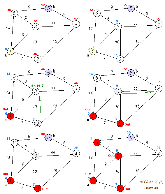
Problem: Write a python function to calculate the shortest path given a start node (or vertex), an end node and a graph. Use Dijkstra’s algorithm. Return the distance from the start node to the end node, as well as the path taken to get there.

The implementation below sticks pretty closely to the algorithm description in the wikipedia entry, which I turned into something a little more pseudo-code-ish to help me implement it:

Initial state:

1. give nodes two properties – node.visited and node.distance
2. set node.distance = infinity for all nodes except the start node which is set to zero.
3. set node.visited = false for all nodes
4. set current node = start node.

Current node loop:

1. if current node = end node, finish and return current.distance & path
2. for all unvisited neighbors, calc their tentative distance (current.distance + edge to neighbor).
3. if tentative distance < neighbor's set distance, overwrite it.
4. set current.isvisited = true.
5. set current = remaining unvisited node with smallest node.distance

Here’s my implementation – it’s recursive, as suggested by the algorithm description:

import sys
def shortestpath(graph,start,end,visited=[],distances={},predecessors={}):
    """Find the shortest path between start and end nodes in a graph"""
    # detect if it's the first time through, set current distance to zero
    if not visited: distances[start]=0
    if start==end:
        # we've found our end node, now find the path to it, and return
        path=[]
        while end != None:
            path.append(end)
            end=predecessors.get(end,None)
        return distances[start], path[::-1]
    # process neighbors as per algorithm, keep track of predecessors
    for neighbor in graph[start]:
        if neighbor not in visited:
            neighbordist = distances.get(neighbor,sys.maxint)
            tentativedist = distances[start] + graph[start][neighbor]
            if tentativedist < neighbordist:
                distances[neighbor] = tentativedist
                predecessors[neighbor]=start
    # neighbors processed, now mark the current node as visited
    visited.append(start)
    # finds the closest unvisited node to the start
    unvisiteds = dict((k, distances.get(k,sys.maxint)) for k in graph if k not in visited)
    closestnode = min(unvisiteds, key=unvisiteds.get)
    # now we can take the closest node and recurse, making it current
    return shortestpath(graph,closestnode,end,visited,distances,predecessors)

if __name__ == "__main__":
    graph = {'a': {'w': 14, 'x': 7, 'y': 9},
            'b': {'w': 9, 'z': 6},
            'w': {'a': 14, 'b': 9, 'y': 2},
            'x': {'a': 7, 'y': 10, 'z': 15},
            'y': {'a': 9, 'w': 2, 'x': 10, 'z': 11},
            'z': {'b': 6, 'x': 15, 'y': 11}}
    print shortestpath(graph,'a','a')
    print shortestpath(graph,'a','b')

    """
    Result:
        (0, ['a'])
        (20, ['a', 'y', 'w', 'b'])
        """

You’ll see I turned the example in wikipedia into a graph for the test case in the code above.

I found this useful about how to represent and process graphs in python: http://www.python.org/doc/essays/graphs.html. I think this was written by Guido himself.

There’s a bunch of interesting implementations on the web, including two here. More elegant, but it took me a while to understand them.

Posted in programming | 6 Comments »

Cyclic Linked List – Python function to find the node at the start of the loop

I’d blogged previously about writing a python function to find out whether a linked list is acyclic or not – it’s worth a read before tackling this one.

Problem: Given the head node of a cyclic (or circular) linked list, write a function to return the node that is at the start of the loop.

A cyclic linked list would look something like this:

A->B->C->D->E->F->C

In the case above, A is the head node, and C is the node at the start of the loop.

My Solution

Let’s call x the distance from the head to the start of the loop, and c the number of nodes in the loop.

We kick off a fast and a slow pointer from the head, with the fast pointer going twice as fast as the slow pointer (skipping every other node). By the time the slow pointer gets to the start of the loop, the fast pointer will have a head start of x (the fast pointer is always the same distance from the slow pointer as the slow pointer is from the head).

Given its head start of x, when will the fast pointer catch up to the slow pointer? The fast pointer always needs twice the initial distance from the slow pointer to catch up. Moving forward in the loop, the fast pointer is c-x nodes from the slow pointer, so it needs 2(c-x) nodes to catch up. In that time, the slow pointer will have managed to move c-x nodes away from the start (half what the fast pointer travelled).

The key thing to note here is that both pointers are now x nodes away from the start of the loop looking in a forwards direction. So you’ll see that to find the start of the loop the code below gets the fast and slow pointer to meet in the loop, then walks the slow pointer forward x nodes – the distance from the head to the start.

def startOfCyclicLoop(head):

    """
    >>> e1=Element(1)
    >>> e2=Element(2)
    >>> e3=Element(3)
    >>> e4=Element(4)
    >>> e5=Element(5)
    >>> e1.next=e2
    >>> print startOfCyclicLoop(e1)
    None
    >>> e2.next=e3
    >>> e3.next=e4
    >>> e4.next=e5
    >>> print startOfCyclicLoop(e1)
    None
    >>> e5.next=e3
    >>> print startOfCyclicLoop(e1)
    3
    >>> e5.next=e4
    >>> print startOfCyclicLoop(e1)
    4
    >>> e5.next=e2
    >>> print startOfCyclicLoop(e1)
    2
    """
    slow=head
    fast=head
    while fast!=None and fast.next!=None:
        slow=slow.next
        fast=fast.next.next
        if (fast==slow):
            slow=head
            while (fast!=slow):
                slow=slow.next
                fast=fast.next
            return fast
    return  None

class Element:
    def __init__(self,data,next=None):
        self.data=data
        self.next=next
    def __str__(self):
        return str(self.data)

if __name__ == "__main__":
    import doctest
    doctest.testmod()

Posted in programming | No Comments »

Puzzle – Hands on a Clock

For a given time, what will be the angle between the hour and minute hands on a clock?

Answer

Posted in puzzles | No Comments »

Anagrams – Python

Write a Python function to find all the anagrams for each of a supplied list of words. For the word dictionary to find the anagrams you could use the one found on Unix or OS X boxes at /usr/share/dict/words. So for example:

>>> for group in anagrams(['dog','cat','horse']):
...     print group
...
['dog', 'god']
['act', 'cat']
['horse', 'shoer', 'shore']

When called without a parameter, make the function return a list of all the anagram groups in the word dictionary, ordered by the group of anagrams with the most words:

>>> for group in anagrams():
...     if len(group)>6: print len(group), group
...
9 ['ester', 'estre', 'reest', 'reset', 'steer', 'stere', 'stree', 'terse', 'tsere']
9 ['angor', 'argon', 'goran', 'grano', 'groan', 'nagor', 'orang', 'organ', 'rogan']
9 ['caret', 'carte', 'cater', 'crate', 'creat', 'creta', 'react', 'recta', 'trace']
8 ['leapt', 'palet', 'patel', 'pelta', 'petal', 'plate', 'pleat', 'tepal']
8 ['laster', 'lastre', 'rastle', 'relast', 'resalt', 'salter', 'slater', 'stelar']
7 ['dater', 'derat', 'detar', 'drate', 'rated', 'trade', 'tread']
7 ['easting', 'gainset', 'genista', 'ingesta', 'seating', 'signate', 'teasing']
7 ['darter', 'dartre', 'redart', 'retard', 'retrad', 'tarred', 'trader']
7 ['least', 'setal', 'slate', 'stale', 'steal', 'stela', 'tales']
7 ['atle', 'laet', 'late', 'leat', 'tael', 'tale', 'teal']
7 ['alem', 'alme', 'lame', 'leam', 'male', 'meal', 'mela']
7 ['lapse', 'salep', 'saple', 'sepal', 'slape', 'spale', 'speal']
7 ['armet', 'mater', 'metra', 'ramet', 'tamer', 'terma', 'trame']
7 ['argel', 'ergal', 'garle', 'glare', 'lager', 'large', 'regal']
7 ['aldern', 'darnel', 'enlard', 'lander', 'lenard', 'randle', 'reland']
7 ['alert', 'alter', 'artel', 'later', 'ratel', 'taler', 'telar']
7 ['arist', 'astir', 'sitar', 'stair', 'stria', 'tarsi', 'tisar']
7 ['aril', 'lair', 'lari', 'liar', 'lira', 'rail', 'rial']
7 ['asteer', 'easter', 'reseat', 'saeter', 'seater', 'staree', 'teaser']
7 ['arpent', 'enrapt', 'entrap', 'panter', 'parent', 'pretan', 'trepan']
>>>

Can you think of an elegant (dare I say pythonic?) way to implement the anagrams function?

Here’s my attempt:

def anagrams(wordsin=None):
    f=open('/usr/share/dict/words')
    ana=dict()
    for word in f.readlines():
        ana.setdefault(''.join(sorted(word.rstrip())),[]).append(word.rstrip())
    if wordsin!=None:
        return [ana.get(''.join(sorted(wordin)),[]) for wordin in wordsin]
    else:
        return sorted(ana.values(), key=lambda(v): (len(v)),reverse=True)

Posted in programming | 2 Comments »

Puzzle – Birthday pairings

Here’s two classic birthday puzzles:

How many people do you need in a room to have a better than 50% chance of finding at least one shared birthday among them?

Answer

How many people do you need in a room with you to have a better than 50% chance of finding someone who shares your birthday?

Answer

Posted in puzzles | 2 Comments »